
The University of Maine The University of Maine
DigitalCommons@UMaine DigitalCommons@UMaine
Non-Thesis Student Work
11-2022
ArcMap Basics: WPES, How Do I...? Quick Guide ArcMap Basics: WPES, How Do I...? Quick Guide
Bea E. Van Dam
University of Maine
Follow this and additional works at: https://digitalcommons.library.umaine.edu/student_work
Part of the Geographic Information Sciences Commons, Hydrology Commons, and the Spatial Science
Commons
Repository Citation Repository Citation
Van Dam, Bea E., "ArcMap Basics: WPES, How Do I...? Quick Guide" (2022).
Non-Thesis Student Work
. 18.
https://digitalcommons.library.umaine.edu/student_work/18
This Article is brought to you for free and open access by DigitalCommons@UMaine. It has been accepted for
inclusion in Non-Thesis Student Work by an authorized administrator of DigitalCommons@UMaine. For more
information, please contact um.library.technical.ser[email protected].
WPES, How Do I…?
Quick Guide to
ARCMAP BASICS

WPES, How Do I…?
Quick Guide to
ArcMap Basics
Prepared by Bea E. Van Dam
for
Watershed Process and Estuary Sustainability Research Group
University of Maine, Orono, ME
umaine.edu/watershedresearch
© 2022 Bea E. Van Dam
ArcMap™, ArcGIS® Desktop, and associated software and extensions are
© 1995-2022 Environmental Systems Research Institute, Inc. (Esri), Redlands,
CA. Microsoft® and Excel® are trademarks of the Microsoft group of
companies.
The “WPES, How Do I…?” series of instruction manuals were originally
developed for internal use by the Watershed Process and Estuary Sustainability
Research Group (WPES) at the University of Maine. They have been updated
and published through DigitalCommons@UMaine to provide open access for
academic use.
Funding support for production of this publication has been provided by the
Maine Agricultural and Forest Experiment Station (MAFES) Project No.
ME0ME022209 and by the Maine Water Resources Research Institute (WRRI)
Project No. 2018ME331B and FY21 Project No. 5520980‐5409118‐20.
This document is formatted for print in booklet form on letter size paper.
i
Table of Contents
Introduction ............................................................................................................. ii
Basic Layout of ArcMap Window .......................................................................... 1
Map Window ...................................................................................................... 1
Table of Contents ............................................................................................... 1
Catalog ................................................................................................................. 1
ArcToolbox ......................................................................................................... 1
Toolbars ............................................................................................................... 3
Importing and Opening Data ................................................................................. 4
Connecting to Folders ........................................................................................ 4
Opening Spatial Data .......................................................................................... 4
Opening Tabular Data ........................................................................................ 5
Querying Data .......................................................................................................... 7
Querying by Attributes ....................................................................................... 7
Querying by Location ......................................................................................... 8
Editing Data ............................................................................................................. 9
Creating New Datasets ....................................................................................... 9
Editing Vector Datasets .................................................................................... 10
Editing Raster Datasets ..................................................................................... 12
Editing Tabular Data ........................................................................................ 15
Exporting Data ....................................................................................................... 18
Exporting Vector Datasets ................................................................................ 18
Exporting Raster Datasets ................................................................................ 19
Exporting Tabular Datasets .............................................................................. 20
Changing Map Appearance .................................................................................. 21
Changing Layer Order ...................................................................................... 21
Changing Layer Symbology ............................................................................. 21
Changing Layer Transparency ......................................................................... 23
Preparing Print Maps ............................................................................................. 23
Layout View ...................................................................................................... 23
Adding Map Elements ...................................................................................... 24
Multiple Map Frames ........................................................................................ 27
Exporting Finished Map ................................................................................... 28

ii
Introduction
This document is a quick guide to performing common geospatial tasks in
ArcMap 10.x (ArcGIS Desktop) for new users. In many cases, there are
multiple ways to accomplish different tasks; presented here are the methods the
author finds easiest or most straightforward. Mouse click sequences and
menu/tool layout may differ if using previous versions of ArcMap. In-depth
official documentation and help topics from Esri are available online at
desktop.arcgis.com/en/arcmap/latest/map.
The University of Maine licenses ArcGIS from Esri for academic use by students
and faculty. ArcGIS may be downloaded for student-owned computers at
umaine.edu/it/software/.
The “Maine Town and Townships Boundary Polygons Feature” (METWP24P)
layer is used for illustration throughout this document. It can be obtained from
the Maine GeoLibrary at maine.gov/geolib/catalog.html.
1
Basic Layout of ArcMap Window
Map Window
This is where your spatial data will appear. The coordinates of your cursor
in the Map Window’s current projection / coordinate system are shown at
the bottom right. Other windows such as the Table of Contents can be
docked along the boundaries of the Map Window by clicking and holding
their title bars and dragging them toward the desired location. Map
Window properties, most importantly the coordinate system, can be
changed by right-clicking in the Map Window and opening the “Data
Frame Properties” dialog.
Table of Contents
From this window you can open and close data layers and change the
appearance of the map by changing the order of opened layers, turning
visibility of layers on and off, and changing layer symbology. If this
window is not showing, it can be opened from the Windows menu in the
File Menu bar or by clicking its icon in the “Standard” toolbar. In Figure 1,
the Table of Contents is in its default “List By Drawing Order” view.
Catalog
From this window you can connect to data folders on your hard drive and
navigate currently connected folders. Data layers can be dragged and
dropped from the Catalog into the Map Window or Table of Contents. If
you delete a data file directly from the Catalog, it does not go to your
computer’s Recycle Bin and cannot be recovered. This window can be
opened from the Windows menu in the File Menu bar or by clicking its
icon in the “Standard” toolbar. In Figure 1, it has been docked on the right
side of the Map Window and set to auto-hide by clicking the pin icon in its
title bar.
ArcToolbox
In this window you can access different toolboxes, collections of interactive
tools for performing specific geospatial analyses and tasks. This window
can be opened from the Geoprocessing menu in the File Menu bar or by
clicking its icon in the “Standard” toolbar.
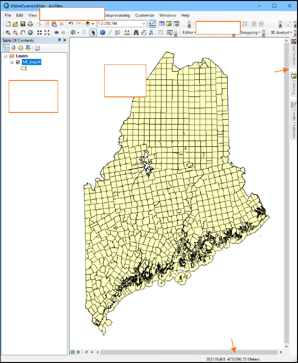
2
Figure 1. Labeled ArcMap window in Data View with one open data layer.
Table of
Contents
Map
Window
Pinned
windows
Cursor
coordinates
Toolbars
File Menu bar

3
Toolbars
Toolbars are collections of tools for performing general tasks in ArcMap.
Toolbars can be turned on and off through the Customize menu in the File
Menu bar or by right-clicking in the Toolbars area above the Map Window.
The “Standard,” “Tools,” and “Editor” toolbars are generally the most
important to have open for everyday tasks, and the “Layout” toolbar should
be open when preparing map documents to print.
Standard
Contains general tools related to opening and saving maps, undoing
and redoing edits, adding data , and setting map cartographic scale,
as well as icons to open other important toolbars and windows.
Tools
Contains tools that work specifically with controlling the view of the
map window, including zoom, pan, view full data extent, and
previous/next view, as well fundamental tools for working with and
exploring spatial data, particularly Select Features (with dropdown
arrow to change the mechanism of selection) and its opposite Clear
Selected Features , Identify , which displays information about
features or raster values, and the Measure tool.
Editor
Contains tools for directly editing vector features, most importantly
the multipurpose Edit Tool .
4
Importing and Opening Data
Connecting to Folders
Unlike most programs, ArcMap has to be explicitly told to access a folder
before data within it can be opened. When a folder has been connected, all
of its subfolders will also be accessible; you may choose to connect directly
to commonly used subfolders in order to reduce the amount of clicking
through layers of subdirectories you must do when connecting to data.
1. Open “Connect To Folder” dialog.
Note: This can be accessed by clicking its icon in the Catalog window -or- through
the Add Data dialog.
2. Navigate to the data folder you wish to connect to.
Note: The C: and D: (if applicable) drives will be under “This PC.”
3. Click “OK.”
Opening Spatial Data
Shapefiles
A
are the basic ArcGIS format for nontopological georeferenced
vector data (points, lines, and polygons) and their associated attribute data.
Raster
B
files are gridded representations of data such as aerial photos or the
LiDAR-derived digital elevation models (DEMs) we commonly work with.
Geodatabases
C
are ArcGIS containers that can hold topological vector
feature, raster, and tabular data.
1. Open “Add Data” dialog.
Note: This can be accessed by clicking its icon in the Standard toolbar -or-
through the File menu under “Add Data” -or- by right-clicking the name of the
active data frame (by default, this is “Layers”) in the Table of Contents.
2. Use dropdown to navigate to folder/geodatabase containing your data.
A
desktop.arcgis.com/en/arcmap/latest/manage-data/shapefiles/what-is-a-shapefile.htm
B
desktop.arcgis.com/en/arcmap/latest/manage-data/raster-and-images/what-is-raster-
data.htm
C
desktop.arcgis.com/en/arcmap/latest/manage-data/geodatabases/what-is-a-
geodatabase.htm
5
3. Click to select desired data file.
Note: To select multiple individual files, hold CTRL while clicking each. To
select range of files, click top file, hold SHIFT, and click bottom file.
4. Click “Add.”
5. Data layer(s) will appear in Table of Contents and Map Window. To
view attribute data for a layer, right-click layer name in Table of
Contents and select “Open Attribute Table.”
Note: Some raster datasets do not contain attribute tables. To access underlying
gridded data for a raster, see Exporting Raster Data section.
Opening Tabular Data
Tabular
D
data files can be opened in ArcGIS even though they are not
directly associated with spatial features. In cases where there are coordinate
columns in the data (e.g., latitude and longitude or northing and easting),
georeferenced spatial features can be created from the data.
Opening Table from Text File
This method directly opens text files (including .csv) for viewing in
ArcGIS.
1. Use “Add Data” dialog to navigate to and select and add
desired data file.
Note: See Opening Spatial Data section.
2. The table and its containing folder will appear in the “List By
Source” view in the Table of Contents. To view table data,
right-click table name in Table of Contents and select “Open.”
Opening Table from Excel File
Microsoft Excel spreadsheets can generally be opened using the same
methods as text files (above), but may not always import correctly.
Below is the more proper method for opening them.
1. Open “Excel to Table” tool in ArcToolbox .
(ArcToolbox > Conversion Tools > Excel > Excel To Table)
D
desktop.arcgis.com/en/arcmap/latest/manage-data/tables/what-are-tables-and-
attribute-information.htm

6
2. For “Input Excel File,” browse to location of file and click
“Open.”
3. For “Output Table,” browse to or type in desired location for new
table to be saved.
4. For “Sheet,” use dropdown to select desired sheet from workbook.
5. Click “OK.”
6. The table and its containing folder will appear in the “List By
Source” view in the Table of Contents. To view table data,
right-click table name in Table of Contents and select “Open.”
Creating Points from Table
1. Right-click table name in Table of Contents and select “Display
XY Data…”
2. For “X Field,” select Easting or Longitude column (as
appropriate) from dropdown menu.
3. For “Y Field,” select Northing or Latitude column.
4. For “Z Field,” select Elevation column if present, otherwise leave
as “<None>.”
5. Select appropriate coordinate system for your data.
Note: See Creating New Datasets section.
5.1. Click “Edit…”
5.2. Navigate through folder structure to coordinate system.
5.3. Click “OK.”
6. Click “OK.”
7. A new point layer named “[YourTableName] Events” will appear
in Table of Contents.
8. Save points in Events layer as new shapefile.
Note: See Exporting Data section.

7
Querying Data
When working with data layers with many features/records, it can be helpful to
be able to find and select records based on their attribute values or on the spatial
location of the features rather than having to select each record manually.
Querying by Attributes
1. Open Selection menu in the File Menu bar and click “Select By
Attributes…”
-or-
With target layer’s attribute table open in “Table” window, click
“Table Options” and choose “Select by Attributes…”
2. In “Layer” dropdown, choose which layer to select records from.
Note: If you opened Select By Attributes window from Table Options in Table
window, this dropdown is unnecessary and does not appear.
3. In “Method” dropdown, choose what type of selection should be
made.
4. Enter query conditions in box under “SELECT * FROM
[LayerName] WHERE:”
Note: The “Help” button below the text box provides a helpful rundown from
Esri of how to format queries in more detail than is provided here.
4.1. To enter a specific attribute column from the table into the
query conditions box, double-click its name in the list below the
“Method” dropdown.
4.2. To select an operator for the query, click its icon or type the
appropriate symbol/word into the query conditions box.
4.3. To see a list of all attribute values that appear in a particular
column within the table, single-click the column name to
highlight it in the list below the “Method” dropdown and click
“Get Unique Values” button.
4.4. To enter a specific unique value into the query conditions box,
double-click its name in the list of unique values.
8
4.5. The simplest type of query selects all records that match a
specific attribute value in a specific column, e.g.,
“COUNTY” = ‘Penobscot’
More complex queries may involve multiple values or conditions,
such as
“COUNTY” IN (‘Penobscot’, ‘Aroostook’, ‘Piscataquis’)
or
“COUNTY” = ‘Penobscot’ AND “ShapeArea” < 100000
5. (Optional) Click “Verify” button to check whether query is valid.
Note: Verification error messages are unfortunately not particularly verbose or
helpful. “A column was specified that does not exist” may mean that double
quotes were put around something other than a proper column name, but also
may mean that a text string value was not enclosed in single quotes. “An invalid
SQL statement was used” may indicate that a numeric value was enclosed in
quotes, or may signify a mismatch between the data type of the specified column
and the operator used, e.g., “COUNTY” > 100 will cause an error if County is a
text attribute column rather than a numeric attribute column.
6. Click “Apply” to run query.
7. When satisfied with query, click “OK” to close Select By Attributes
dialog.
8. To create a new layer from a selection, right-click the source layer in
the Table of Contents and choose “Selection” > “Create Layer from
Selected Features.”
Querying by Location
1. Open Selection menu in the File Menu bar and click “Select By
Location…”
2. In “Selection method” dropdown, choose what type of selection
should be made.
3. Under “Target layer(s),” check the boxes of all layers you wish to select
features from.
4. In “Source layer” dropdown, choose the layer you wish to use as the
basis or comparison against which to select from the target layer.
Note: If the plain-language version of an intended query is “Select all towns
within 25 km of Bangor,” the Target layer is the layer containing all towns,
while the Source layer is a layer or selection containing only the city of Bangor.

9
5. In “Spatial selection method for target layer feature(s)” dropdown,
choose which measure of proximity the Target layer features should
have to the Source features.
5.1. For some selection measures such as “are within a distance of the
source feature,” you must specify the search distance. For some
other selection measures, applying a search distance is optional.
6. Click “Apply” to run query.
7. When satisfied with query, click “OK” to close Select By Location
dialog.
8. To create a new layer from a selection, right-click the source layer in
the Table of Contents and choose “Selection” > “Create Layer from
Selected Features.”
Editing Data
Creating New Datasets
Users may use the Catalog to create new empty datasets in which they can
add new data. Most commonly, these will be vector datasets to hold points,
polylines, or polygons. If creating a raster or tabular dataset, some details
may differ from the steps outlined below.
1. Open Catalog window and navigate to folder in which you wish
to create new dataset.
2. Right-click folder and select “New” > “Shapefile” to open “Create
New Shapefile” dialog.
Note: If working in a geodatabase, the equivalent is vector file type is “Feature
Class.” Feature classes have a slightly more involved creation dialog but share
with shapefiles the same three mandatory fields described below.
3. Enter name for new layer.
4. Use dropdown to select feature type for new layer.
5. Click “Edit…” to open “Spatial Reference Properties” dialog.

10
5.1. Navigate through folder structure to select appropriate
coordinate system
E
.
Latitude/Longitude:
• (Commonly) World Geodetic System (WGS) 1984 –
Geographic Coordinate Systems > World > WGS 1984
• (Occasionally) North American Datum (NAD) 1983 –
Geographic Coordinate Systems > North America > USA
and territories > NAD 1983
Northing/Easting:
• (Commonly) Universal Transverse Mercator (UTM)
projection (Zone 19 for Maine) – Projected Coordinate
Systems > UTM > NAD 1983 > NAD 1983 UTM Zone
19N
• (Rarely) State Plane survey projection – Projected
Coordinate Systems > State Plane > NAD 1983 (Meters)
> NAD 1983 Maine 2000 [East\Central\West] Zone
(Meters)
Note: If your state plane Northing/Easting coordinates are in
feet, substitute “NAD 1983 (US Feet)” folder.
5.2. Click “OK.”
6. Click “OK.”
7. Newly created layer will be added to Table of Contents and may be
edited using steps in following section.
Editing Vector Datasets
Spatial components of vector datasets (shapefiles and geodatabase feature
datasets containing points, lines, or polygons) may be edited directly (e.g.,
by moving individual vertices) with the Editor toolbar. Additionally, more
complex automated tasks can be performed using tools from the
ArcToolbox, most of which output a separate new vector dataset at the end
of the operation. Instructions for these tools are not included here, but
several common operations can be explored within the “Analysis Tools”
toolbox.
E
desktop.arcgis.com/en/arcmap/latest/map/projections/what-are-map-projections.htm

11
Editor Toolbar
1. Ensure Editor toolbar is turned on/visible.
2. Open Snapping toolbar (“Editor” dropdown > “Snapping”) and
set desired snapping behaviors.
Note: Snapping allows nodes to be placed precisely coincident with existing
vertices, intersections, and shape or line edges
3. Right-click vector layer to be edited in Table of Contents and
select “Edit Features” > “Start Editing.”
Note: This makes all vector data layers in the same geodatabase or file
folder editable. To avoid inadvertent edits to other layers, it can be helpful
to turn them off in the Table of Contents.
4. To manipulate vertices in existing features:
4.1. Double-click feature using Edit Tool to enter “Edit
Vertices” mode.
4.2. Use Edit Tool to select individual vertices by clicking or drag
a bounding box to select multiple vertices.
4.3. Click and hold on selected vertex and drag to reposition.
4.4. Add or Delete vertices using tools in Edit Vertices
toolbar.
4.5. Click outside the feature to exit “Edit Vertices” mode.
5. To add new features:
5.1. Open “Create Features” editing window (“Editor”
dropdown > “Editing Windows”).
5.2. Click name of editable layer in “Templates” panel (top part
of Create Features window).
5.3. Click desired feature type in “Construction Tools” panel
(bottom part of Create Features window).
5.4. In Map Window, click each location where you wish to
place a new feature vertex. To end a new line or polygon,
double-click final vertex location.
6. To copy an existing feature into an editable layer:
6.1. Select feature(s) with Edit Tool .

12
Note: Feature to be copied may be in either an editable or non-
editable layer.
6.2. Right-click in Map Window and select “Copy” or use
keyboard shortcut CTRL+C to copy feature.
6.3. Right-click in Map Window and select “Paste” or use
keyboard shortcut CTRL+V to paste feature into editable
layer.
6.3.1. If there are multiple editable layers with the
compatible feature type, select the correct layer from
the “Target” list in the pop-up Paste dialog.
7. To combine multiple features in the same editable layer:
Note: This option is only available with line and polygon features, not
points.
7.1. Select features with Edit Tool .
Note: Hold Shift key while clicking each.
7.2. Open “Editor” dropdown and select “Merge.”
7.3. In “Merge” dialog, select feature into which the other
feature(s) will be merged and click “OK.”
Note: Attribute data for the target feature will be retained in the
attribute table, while attribute data for the other input feature(s)
will be lost.
8. To undo an edit, click “Undo” icon in Standard toolbar or use
keyboard shortcut CTRL+Z.
9. To save edits at any point, open the “Editor” dropdown and select
“Save Edits.”
10. When finished editing, open the “Editor” dropdown and select
“Stop Editing.”
Editing Raster Datasets
Raster datasets cannot be directly edited in ArcMap and must instead be
manipulated using tools from the ArcToolbox, most of which output a
separate new raster at the end of the operation. Following are instructions
for two of the most common editing operations.
13
Merging Rasters
Used for combining multiple adjacent rasters such as Digital Elevation
Model (DEM) tiles, or for overwriting values in one raster with values
from an overlapping raster.
1. Open “Mosaic to New Raster” tool – Data Management Tools >
Raster > Raster Dataset
2. Use dropdown or browse to select input rasters to be merged.
3. Browse to select output location and click “Add.”
4. Enter desired output dataset name and extension.
Note: We most commonly use the TIFF format, extension “.tif”. If no
extension is specified, output will be saved as a “File System Raster” if saved
to a normal file system folder. Any output saved to a geodatabase will be
saved as a “Geodatabase Raster Dataset;” specifying an extension may
result in that extension alone being used as the file name.
5. Browse to desired spatial reference (coordinate system) for
output.
Note: Spatial references for data layers can be found in their Layer
Properties under the “Source” tab. See also pg. 6, Creating Points from
Table.
6. Use dropdown to select Pixel Type.
Note: This value refers to the amount and type of data that can be stored as
a cell value and should generally correspond to the largest pixel depth of the
input rasters. Pixel depths for data layers can be found in their Layer
Properties under the “Source” tab.
7. Enter number of bands of data in raster output.
Note: This is effectively the number of separate values each raster cell may
hold, and may be no more than the minimum number of bands among the
input rasters. For satellite imagery and other photo rasters, the number of
bands is generally three or more (for Red, Green, Blue, and occasionally
Gamma or other data), while elevation rasters generally have only one
band.
8. Use dropdown to set mosaic operator.
Note: ArcMap defaults to “Last,” in which the value for any cell is taken
from that of the last overlapping raster listed among the input rasters (step
2). For merging adjacent tiled rasters this is relatively unimportant, but
14
when updating one raster with values from another the correct order is
crucial.
9. Click “OK.”
Clipping Raster
Used for cropping rasters to a specified extent using a bounding box or
other spatial data layer.
1. Open “Clip” tool – Data Management Tools > Raster > Raster
Processing.
2. Use dropdown or browse to select input raster to be clipped.
3. Output extent may be specified in one of two ways:
3.1. Enter bounding coordinates directly in X and Y Minimum
and Maximum boxes
-or-
3.2. Use dropdown or browse to select existing polygon layer to
clip to.
Note: If layer chosen from the dropdown has an active selection, the
tool will clip to only the selected features, not the entire layer.
3.2.1. Optionally, check “Use Input Features for Clipping
Geometry” box.
Note: If this box is not checked, the tool will populate the
bounding coordinate boxes with the minimum bounding
rectangle surrounding the polygon layer features and not
clip to the edges of the polygon features.
4. Browse to desired output location.
4.1. Enter desired output dataset name with extension.
Note: We most commonly use the TIFF format, extension “.tif”. If
no extension is specified, output will be saved as a “File System
Raster” if saved to a normal file system folder. Any output saved to a
geodatabase will be saved as a “Geodatabase Raster Dataset;”
specifying an extension may result in that extension alone being used
as the file name.
4.2. Click “Save.”
5. Click “OK.”
15
Editing Tabular Data
ArcMap is inconsistent in the way it allows editing of tabular data,
including attribute tables of vector and raster layers. Common operations
are outlined below.
All operations begin with right-clicking layer or table name in Table of
Contents and selecting “ Open [Attribute Table]” to open Table
window.
Note: Not all table types may be edited. Existing text (including .csv) and Excel files
that have been opened for viewing in ArcMap through the Add Data dialog may not
be edited; editable versions can be created by exporting the data (see Exporting
Tabular Datasets).
Not all raster layers will have attribute tables.
Adding New Column
1. For this operation, table or layer must not be in an active edit
session.
2. With table open in Table window, click “Table Options” icon
and click “Add Field…” to open Add Field dialog.
3. Enter name for new field.
Note: Column names are limited to ten characters in length.
4. Use dropdown to select type of data the new column will hold.
5. Click “OK.”
Deleting Column
1. For this operation, table or layer must not be in an active edit
session.
2. With table open in Table window, right-click column to be
deleted and click “Delete Field.”
3. If and only if you wish for the field and all its data to be
permanently and irretrievably deleted, confirm deletion by
clicking “Yes.”

16
Adding New Row
Note: New rows added to a feature layer through this method will be created
without an associated spatial feature (point/line/polygon). The spatial feature
can be added later (Editor Toolbar > Edit Vertices > Continue Feature Tool),
but this is an uncommon workflow.
1. Right-click table or layer to be edited in Table of Contents and
select “Edit Features” > “Start Editing.”
2. With table open in Table window, scroll to blank row at bottom
of table.
3. In blank row, click empty cell under non-keyword column (i.e.,
not “OBJECTID” or “FID”) and enter desired column attribute
value for new record.
3.1. Any other numeric fields in the row will auto-populate with
“<Null>” (for tables saved in geodatabase) or “0”.
4. Continue entering attribute values for other columns in row.
5. To save edits at any point, open the “Editor” dropdown in Editor
toolbar and select “Save Edits.”
6. When finished adding and populating new rows, open the
“Editor” dropdown and select “Stop Editing.”
Deleting Row
Note: Deleting row in a feature layer will also delete associated spatial feature
(point/line/polygon).
1. Right-click table or layer to be edited in Table of Contents and
select “Edit Features” > “Start Editing.”
2. With table open in Table window, select desired row by clicking
box to left of first column.
Note: To select multiple rows, hold CTRL key while clicking each, or to
select a contiguous block of rows click the topmost selection, hold SHIFT, and
click the bottommost.
3. Click “Delete Selected” icon.
4. To save edits at any point, open the “Editor” dropdown in Editor
toolbar and select “Save Edits.”

17
5. When finished editing, open the “Editor” dropdown and select
“Stop Editing.”
Updating Single Cell Value
1. Right-click table or layer to be edited in Table of Contents and
select “Edit Features” > “Start Editing.”
2. With table open in Table window, click cell you wish to edit.
3. Enter desired new value.
4. To undo an edit, click “Undo” icon in Standard toolbar or use
keyboard shortcut CTRL+Z.
5. To save edits at any point, open the “Editor” dropdown in Editor
toolbar and select “Save Edits.”
6. When finished editing, open the “Editor” dropdown and select
“Stop Editing.”
Updating Column with Formula
Values for an entire column may be updated at once using a formula.
This operation may be used to populate all rows in the column with a
single value or with new unique values based on attributes in other
columns (e.g. [Column_A]+[Column_B]-[Column_C]).
If there is an active selection in the table, updates will be applied only
to selected records, not to all records in table.
1. For this operation, table or layer may or may not be in an active
edit session.
Note: If the table is currently editable, unwanted or erroneous column
updates may be undone until editing session is ended. If operation is
performed while table is not in an editing session any changes may not be
reverted – any previous values are permanently lost.
2. With table open in Table window, right-click name of column
you wish to update and select “Field Calculator.”
3. In Field Calculator window, enter formula in
“[ColumnName] =” text box.
3.1. To incorporate values from another column, double-click
column name in “Fields:” list.
18
3.2. Text strings must be enclosed in quotation marks.
4. Click “OK.”
Updating Column with Geometry
Note: This operation is available only for vector layers with spatial features.
Values for an entire column may be updated at once based on feature
geometry (e.g., point coordinates, line length, or shape area).
If there is an active selection in the table, updates will be applied only
to selected records, not to all records in table.
1. For this operation, layer may or may not be in an active edit
session.
Note: If the layer is currently editable, unwanted or erroneous column
updates may be undone until editing session is ended. If operation is
performed while table is not in an editing session any changes may not be
reverted – any previous values are permanently lost.
2. With attribute table open in Table window, right-click name of
column you wish to update and select “Calculate Geometry.”
3. In Calculate Geometry window, use “Property:” dropdown to
select geometry attribute you wish to populate column with.
4. Use radio buttons to select which coordinate system to use for
calculation.
5. Use “Units:” dropdown to select units for value calculation.
6. Click “OK.”
Exporting Data
Exporting data is analogous to the “Save As…” function of many programs
and is most often done to convert an existing data layer to a different
format or to create a new file containing a subset of an existing dataset (e.g.,
a selection or query).
Exporting Vector Datasets
1. Right-click vector layer to be exported in Table of Contents and select
“Data” > “Export Data” to open Export Data dialog.
19
2. Use drop-down to choose whether to export all features in the layer,
only selected features (if any selection is active), or only features
currently within the visible area of the map window.
Note: Before entering the Export Data dialog, a subset of features may be selected
manually using the Select Features tool in the map window or through the
Select by Location or Select by Attribute dialogs under the Selection menu in the
File Menu bar.
3. Use radio buttons to choose whether exported data will use coordinate
system of the original dataset or that of the data frame.
4. Browse to desired output location.
4.1. Use dropdown to select output file type (most commonly
Shapefile or File and Personal Geodatabase feature).
Note: Geodatabase feature classes may only be saved into geodatabases,
while shapefiles may only be saved into normal file folders. Geodatabases
will not appear in file tree if “Save as type” is set to Shapefile.
4.2. Enter desired file name.
4.3. Click “Save.”
Note: If an “Error Saving Object” pop-up message appears, ensure you are
not trying to save a geodatabase feature class into a file folder.
5. Click “OK.”
Exporting Raster Datasets
As Spatially Referenced Raster
1. Right-click raster layer to be exported in Table of Contents and
select “Data” > “Export Data” to open Export Data dialog.
2. Under “Extent,” use radio buttons to select whether to export the
entire raster dataset, only the portion currently showing in the
data frame (map window), or only the portion within a selected
graphic.
Note: The selected graphics (clipping) option requires the user to have
drawn a polygon using the Draw toolbar. To clip rasters to features from
an existing data layer, see Editing Raster Datasets section.
3. Under “Spatial Reference,” use radio buttons to choose whether
exported data will use coordinate system of the original raster or
that of the data frame.
20
4. (Uncommon) Under “Output Raster,” make desired changes to
output cell size (in map units) and “NoData” (null cell) value.
5. Browse to desired output location and click “Add.”
6. Use “Format” dropdown to select output file type.
Note: We most commonly use the TIFF format. If selected output file
location is a geodatabase, output file format will be automatically set to
File Geodatabase.
7. Enter desired file name.
8. Click “Save.”
Underlying Data Only
While many statistical analyses on raster datasets can be run directly in
ArcMap using tools included in the ArcToolbox, it may be
occasionally desirable to export only the underlying gridded data values
from a raster for analysis outside of ArcGIS (e.g., in Python or R).
Output file is a space-delimited ASCII text file with six header rows
describing the data followed by a number of data rows equal to the
number of rows in the raster image.
1. From ArcToolbox , open “Conversion Tools” > ”From
Raster” > ”Raster to ASCII.”
2. Use dropdown or browse to select input raster to be exported.
3. Browse to desired output location.
3.1. Enter desired file name.
3.2. Click “Save."
Exporting Tabular Datasets
1. Right-click table to be exported in “List By Source” view of Table
of Contents and select “Data” > “Export Data” to open Export Data
dialog.
-or-
With table open in “Table” window, click “Table Options” and
select “Export.”

21
Note: The latter allows you to export attribute tables, if present, from vector or
raster layers without the accompanying spatial data.
2. Under “Export,” use dropdown to choose whether to export all
records in the table or only selected records (if a selection is active).
3. Browse to desired output location.
3.1. Use dropdown to select output file.
Note: Geodatabase tables may only be saved into geodatabases.
Geodatabases will not appear in file tree if “Save as type” is not set to
geodatabase table type.
3.2. Enter desired file name.
3.3. Click “Save.”
Note: If an “Error Saving Object” pop-up message appears, ensure you are
not trying to save a geodatabase table into a file folder.
4. Click “OK.”
Changing Map Appearance
Changing Layer Order
Spatial data layers in the Map Window are drawn in order of appearance in
the “List By Drawing Order” view of the Table of Contents, with layers
at the top of the list drawn above (overlaying) those lower on the list.
Layers can be dragged and dropped in the desired order.
Changing Layer Symbology
1. Right-click layer name in Table of Contents and select “Properties” to
open Layer Properties dialog.
2. Click “Symbology” tab.
3. In “Show:” list at left, select type of symbology, then make desired
adjustments.
Note: See Vector Layers and Raster Layers below for explanation of most
commonly used symbology types.
4. To preview updated symbology, click “Apply.”
5. To finalize symbology change, click “OK.”
22
Vector Layers
• “Features” displays all features in the layer with the same symbol.
To change appearance of that symbol, click the symbol (to right)
to open Symbol Selector and make desired style adjustments.
• “Categories” displays features with different symbology using
categorical (qualitative) groupings based on unique values from
one or more attribute columns specified under “Value Field.”
Symbol color can be adjusted for each included value individually
by clicking symbol or for all values using one of many preset
Color Ramps.
• “Quantities” displays features in multiple ordered classes based on
numeric values from an integer or float datatype attribute column
specified under “Value” field. Data may be classified into equal
intervals (max – min / #classes), defined intervals (e.g., by 5s), or
other standard class type, or users can manually set break values
between ranges.
Raster Layers
• “Unique Values” displays cells with different colors based on
unique cell values. This is appropriate for categorical (qualitative)
data like land cover type. Cell color can be adjusted for each
included value individually by clicking symbol or for all values
using one of many preset Color Schemes.
• “Classified” displays cells in multiple ordered classes based on
numeric cell values. Data may be classified into equal intervals
(max – min / #classes), defined intervals (e.g., by 5s), or other
standard class type, or users can manually set break values between
ranges.
• “Stretched” displays cells with colors stretched along a color ramp
(vs. in discrete classified ranges) based on numeric cell values.
This is appropriate for continuously varying data fields such as
digital elevation models. Distribution of values along the color
ramp can be adjusted by changing “Stretch Type.”

23
Changing Layer Transparency
Layers may be made semitransparent in order to allow underlying data to
show through without entirely turning off the overlying layer.
1. Right-click layer name in Table of Contents and select “Properties” to
open Layer Properties dialog.
2. Click “Display” tab.
3. Enter desired value in Transparency field.
Note: For vector layers, the field is labeled “Transparent.”
4. Click “OK.”
Preparing Print Maps
Users may need to prepare finished maps for print or for online display,
such as for sharing visualized data with colleagues or stakeholders. An in-
depth discussion of the philosophy and practice of effective cartographic
design is beyond the scope of this manual,
F
but following is a basic overview
of how to construct map layouts in ArcMap and the elements that should
be included in most maps.
Layout View
To this point, we have been working in ArcMap’s default “Data View.”
Print maps are instead prepared in the Layout View, which is opened from
the “View” menu in the File Menu bar.
The Layout View shows a stylized sheet of paper on which the map and
other elements can be arranged. Elements can be selected, dragged and
dropped, and resized using the Select Elements tool in the Tools toolbar.
A thin dashed line running just inside page border marks the edge of the
printable area. To change paper orientation (landscape vs portrait) or size,
F
For a short primer on map design principles, see e.g.
esri.com/news/arcuser/0112/make-maps-people-want-to-look-at.html
24
right-click in the white space just outside the page boundaries and select
“Page and Print Setup.”
Adding Map Elements
In addition to the spatial data visualization (i.e., the “map” itself), map
layouts should carry certain other information to clarify and contextualize
the map data. The elements below are added using the “Insert” menu in
the File Menu bar. Other basic shapes and text can also be added to the
layout using the Draw toolbar. In the included example map (Figure 2),
map elements are arranged in white space within the borders of the map
frame; when spatial data extends to the edges of the map frame it is often
preferred to place elements in a separate bar above or below the map frame.
Title
Insert > Title or Insert > Text
Maps should be given a concise title that conveys their main focus or
purpose. A subtitle can be added as a second text element. Text can be
changed and font updated by double-clicking text element or right-
clicking element and selecting “Properties."
North Arrow
Insert > North Arrow
A north arrow allows the user to properly orient the map. This is
particularly important on maps where north is not at the top of the
page, in which case the north arrow should be rotated by the
appropriate angle under “Properties” in the North Arrow Selector. If
arrow is oriented to magnetic rather than true north, a separate text
element to that effect should also be included adjacent to the arrow
(this may be as simple as placing an “M” before the “N” of the arrow).
25
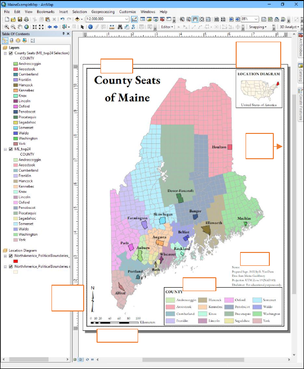
Figure 2. ArcMap window in Layout View showing a simple thematic
(categorical symbology) map layout with important map elements labeled. When
designing maps, consider their accessibility for different viewers – this example
labels the county seats but relies on color to identify associated county names,
making it less accessible to readers with certain types of colorblindness and those
who are seeing a copy printed in grayscale (as some of you may be experiencing
right now).
Title
North
Arrow
Scale Bar
Legend
Notes
Neat
Line
Location
Diagram

26
Scale Bar
Insert > Scale Bar
A scale bar provides a visual representation comparing units of
distance in the real world to their corresponding representation on the
page. Unlike scale text (“1:24,000,” “1 cm = 5 km,” etc.), a scale bar is
accurate even when an image of the map layout is reproduced at a
different size than the original (e.g., enlarged to fit on a poster or
shrunk to fit in a booklet). Properties such as number of divisions,
division length, bar height, and fonts can be customized from the Scale
Bar Selector dialog.
If working with multiple map frames, the scale bar will correspond to
whichever frame is active when the scale bar is inserted (see Multiple
Map Frames). Be sure to activate the correct map frame before
inserting a scale bar, and place the bar in a location that makes it clear
which map it is associated with (often in a lower corner of the
appropriate map frame).
Legend
Insert > Legend
Legends explain the symbology used in the map, making them perhaps
the most important element to include in your layout. From within
the Legend Wizard, you may choose which map layers to show in the
legend, adjust their arrangement, and change fonts and other
formatting. For an in-depth explanation of the extensive legend
customization options, see Esri’s documentation
G
.
To change the way layer names and symbology labels appear in the
legend, right-click layer name in the Table of Contents and select
“Properties.” Layer Name may be updated in the “General” tab and
symbol description may be updated in the “Symbology” tab under the
“Label” field.
G
desktop.arcgis.com/en/arcmap/latest/map/page-layouts/working-with-legends.htm

27
Notes
Insert > Text
Maps should include some basic information about how they were
produced, including cartographer name, production date, and sources
if using data you did not produce yourself. For maps involving any
type of spatial measurement, include the projection/datum the data are
visualized in. For liability purposes it is also recommended to include a
short disclaimer outlining intended uses and limitations of the map.
Neat Line
Insert > Neatline
A neat line is a border enclosing the various map elements inside the
layout margins. Neat lines are occasionally omitted for stylistic
reasons, but generally give a more professional look to the layout.
Location Diagram
See Multiple Map Frames
It is often useful to contextualize your spatial data by including an
additional map frame that shows the location of your mapped area in
relation to a more easily recognized boundary, such as a town, county,
state, or country. If your map depicts an area or feature that your
intended audience will recognize by sight (such as the State of Maine in
Figure 2), the location diagram may not add useful context and is not
strictly necessary.
Multiple Map Frames
It is sometimes necessary or desirable to show multiple maps in the same
layout, such as to include a location diagram or an inset map showing
additional detail for a small area. A second map frame can be added via File
Menu bar > Insert > Data Frame. This will add a blank data frame
(labeled “New Data Frame”) to the map layout and to the Table of
Contents. Like the default data frame (labeled “Layers” in the Table of
Contents), layers can be added using the Add Data dialog and
manipulated as described throughout this manual. Layers can also be
dragged from one frame in to another, which maintains their symbology.

28
When working with multiple data frames, only one can be active for
manipulation at a time. From the Layout View, simply click the desired
data frame with the Select Elements tool to activate it. If working in the
Data View, right-click the data frame name in the Table of Contents and
select “Activate.”
Exporting Finished Map
Electronic versions of the map layout may be saved by opening the File
menu in the File Menu bar and selecting “Export Map.” Outputs may be as
a variety of image file format (e.g., PNG, BMP, etc.) or as a PDF.
Paper copies of the map layout may be printed by opening the File menu
and selecting “Print.” The “Setup” option in the Print dialog allows the
user to select a printer and choose print options as well as to print to PDF.
